This project page demonstrates the detailed descriptions of data and modeling techniques introduced in the poster submitted to the ISSP 2020 as a supplement.
Introduction
Variability is inherent in skilled human motor movements. Playing a piano or riding a bicycle requires skilled coordination of motor elements, such as arms and legs, to achieve a motor goal. Although the movements are skillful, the positions of the motor elements are not exactly the same regardless of how many times they are repeated or executed (“repetition without repetition”; Bernstein, 1967). This variability in the form of repeated limb movements can be understood as an informative biological feature in the human motor system due to its underlying structure and regularity (Latash et al., 2002; Riley & Turvey, 2002; Sternad, 2018; Whalen & Chen, 2019), which previously had been disregarded as noise. One such structure of the skilled motor movements is that it is highly synergistic and flexibly organized when decomposed into “good” and “bad” parts of variability (i.e., the uncontrolled manifold approach or the UCM; Latash et al., 2002; Scholz & Schöner, 1999, 2014). Whether variability in speech production can also be decomposed into the same principle, however, has been rarely examined to date. Specifically, this project aims to focus on the "good" part of variability in speech production and explore the use of invertible neural networks as a quantitative approach to understand how "good" variability is structured and can be learned by these neural-net models.
Data
The Haskins IEEE rate comparison database (Sivaraman et al., 2015; henceforth, the EMA-IEEE database) were utilized
for the UCM analysis and FlowINN modeling. This database includes simultaneous articulatory and
acoustic recordings from eight native American English speakers (4 females, 4 males).
The articulatory data were collected using electromagnetic articulography (EMA), where eight pellet sensors,
sampled at 100 Hz, were attached to speakers’ articulators and later corrected for head movements.
Synchronous acoustic data were recorded at a sampling rate of 44.1 kHz.
Speakers read 720 phonetically balanced sentences at both a normal and a fast rate,
providing various consonant contexts to examine at both rates across speakers.
Nine English vowels (/i, ɪ, ɛ, æ, ʌ, ɔ, ɑ, ʊ, u/) will be selected for the modeling
of the forward mapping functions, while four front vowels (/i, ɪ, ɛ, æ/)
representing vertical articulatory movement were focused on in the analysis.
Data preprocessing steps includes data normalization and dimension reduction.
The purpose of normalizing articulatory and acoustic data was to account for individual differences
as well as differences in the ranges of values and units (millimeter versus frequency).
For articulatory data, six pellet sensors (with two horizontal and vertical sagittal coordinates per sensor)
were selected: TR (Tongue Root), TB (Tongue Body), TT (Tongue Tip), UL (Upper Lip), LL (Lower Lip) and JAW.
Twelve-dimensional kinematic data (six sensors with x-y coordinates) were Z-scored by speaker and then
reduced down to three principal components (PCs) using the principal component analysis that
roughly reflects the vertical, horizontal and residual movement of articulators.
For acoustics data, the first two formant frequencies (F1, F2) were used and also normalized by speaker
using the Z-scoring method. For each vowel, both articulatory and acoustic data were extracted at nine equidistant
and normalized time points in which the 5th time point was the mid-point.
Outliers were identified and removed prior to data normalization in order to reduce noise in the data.
This data normalization procedure followed the guidelines taken from Whalen et al. (2018).
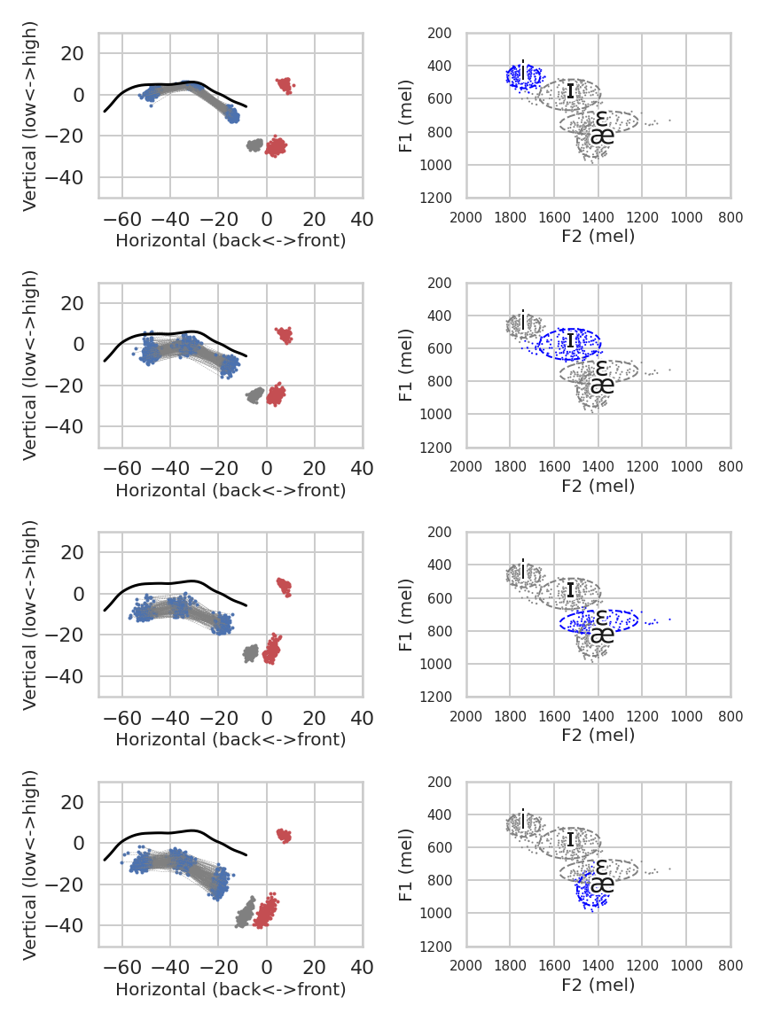
The following plots demonstrate a single speaker (F01)'s vowel production data at normal rate. The first four-by-two plots
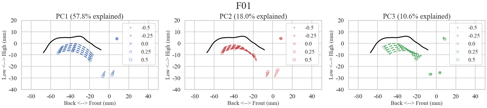
visualize vowel-by-data of the corresponding articulation and acoustics. The bottom plots shows the effects of moving along the
Principal Component dimensions from the same speaker as an example.
Articulatory and acoustic data for the four front vowels /i, ɪ, ɛ, æ/ of speaker F01
Synthesis along the first three Principal Components in articulatory data from speaker F01
Methods
For the mapping between articulation and acoustics, we borrowed the INN model architectiure from Ardizzone et al. (2019), but further customized for our purpose. The input data (\(x\)) was 3-D articulatory vector from the dimension-reduced Principal Components from the EMA sensor coordinates. The output data (\(y\)) was 2-D acoustic vector; that is, the first two formant frequencies (F1, F2). The dimension of the latent space was set to 2-D and appended to \(y\). The total dimensions were set to 6, which led to padding both on the input (\(6 - 3 = 3)\) and outputs (\(6 - 4 = 2)\). Given that \(\mathbf{x} \in \mathbb{R}^{3}\), \( \mathbf{y} \in \mathbb{R}^{2} \) and \( \mathbf{z} \in \mathbb{R}^{2} \), the forward mapping model \(f\) and its inverse \( f^{-1}=g \) can be written as follows (Note that \(\theta\) is neural-net parameters):
Forward process: \( [\mathbf{y}, \mathbf{z}] = f(\mathbf{x}; \theta) \)
Inverse process: \( \mathbf{x} = g(\mathbf{y}, \mathbf{z}; \theta), \, \mathbf{z} \sim \mathcal{N}(\mathbf{z}; 0, I_{2}) \)
Both forward and inverse processes share the same neural network parameters \( \theta \) and implemented in a single invertible neural-net model. Using these definitions, the current INN model for articulation and acosutics can be expressed in a following manner using the change-of-variable technique.
\( p(\mathbf{x}) = p(\mathbf{x} = g(\mathbf{y}, \mathbf{z}; \theta)) \left| det \left( \frac{\partial g(\mathbf{y},\mathbf{z};\theta)}{\partial[\mathbf{y},\mathbf{z}]} \right) \right|^{-1} \)
We used the simplest affine coupling layer structured as described in Dinh et al. (2014); therefore, the computation of the Jacobian determinant was simple because each layer was volume-preserving transformation setting the determinant to one. The structure of the affine coupling layers was first to split \(x\) into two blocks (\( x_1, x_2 \)) and to apply blocks of transformaions from (\( x_1, x_2 \)) to (\( y_1, y_2 \)) as follows.
\( \begin{eqnarray*} y_1 &=& x_1 \\ y_2 &=& x_2 + m(x_1). \end{eqnarray*} \)
The \( m \) was implemented as multilayer perceptrons (MLP) with rectified linear unit (ReLU) activations. Because this forward mapping has a unit Jacobian determinant for any \( m \), the inverse was trivially found.
\( \begin{eqnarray*} x_1 &=& y_1 \\ x_2 &=& y_2 - m(y_1). \end{eqnarray*} \)
The actual TensorFlow2 implementation of the model architecture is summarized as below.
Model: "NICECouplingBlock"
_________________________________________________________________
Layer (type)                 Output Shape              Param #
=================================================================
layer0 (AdditiveAffineLayer) (None, 6)                 981
_________________________________________________________________
layer1 (AdditiveAffineLayer) (None, 6)                 981
_________________________________________________________________
layer2 (AdditiveAffineLayer) (None, 6)                 981
_________________________________________________________________
layer3 (AdditiveAffineLayer) (None, 6)                 981
_________________________________________________________________
layer4 (AdditiveAffineLayer) (None, 6)                 981
_________________________________________________________________
ScaleLayer (Scale)           (None, 6)                 6
=================================================================
Total params: 4,911
Trainable params: 4,881
Non-trainable params: 30
_________________________________________________________________
Results
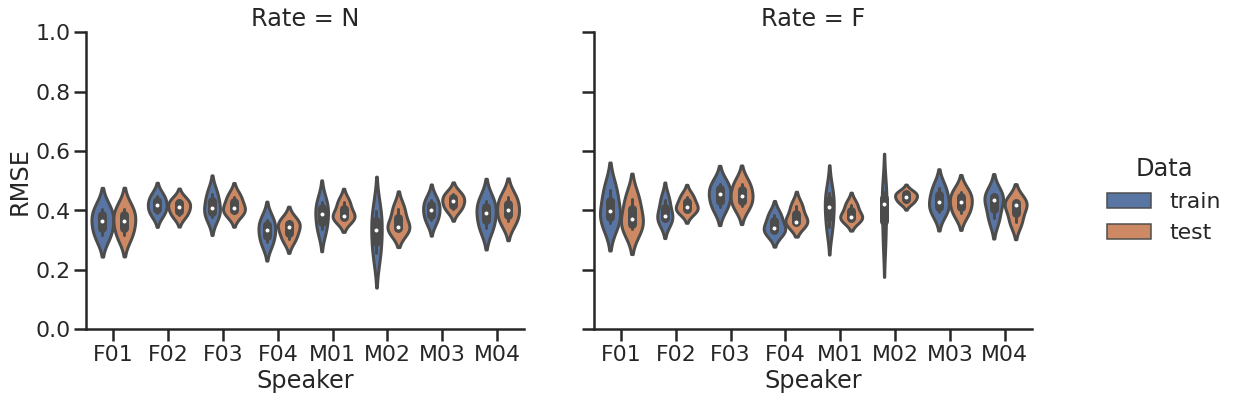
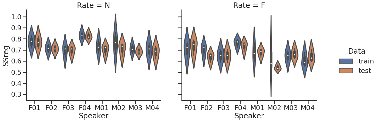
The modeling result is summarized in the following two plots. The top plots demonstrates the root mean-squared error (RMSE) by speaker and rate. Overall, the pattern is similar, but normal-rate models are slightly better than the fast-rate models, possibly because of the smaller variability in the normal-rate data. The bottom plots illustrates how much variability is explained by the model as the index of the sum-of-squared regression (SSreg). Despite the individual differences, the normal-rate models are generally better at explaining the variability in the data.
The Root Mean-Squared Error by speaker (total 8) and speaking rate (N vs. F)
The Sum-of-Squared regression by speaker (total 8) and speaking rate (N vs. F)
The result of forward and inverse mapping with latent-space sampling is visualized in the following plots. You can select different Speaker, Rate and Vowel in the dropdown menu. The plots will change accordingly.
1. Forward and inverse mapping between articulation and acoustics
↓↓ Please choose Speaker, Rate and Vowel from the dropdown menus to see the result.
Speaker:Rate:
Vowel:
2. Forward and inverse mapping between acoustics and vowel categories
↓↓ Please choose Speaker, Rate and Vowel from the dropdown menus to see the result.
Speaker:Rate:
Vowel:
Summary & Conclusion
Language is produced by movement. The articulatory movement in speech accompanies a substantial amount of variability, like any other skilled human behavior. The current project aimed to examine how such variability is structured and can be modeled using flow-based invertible neural networks. This work is still in progress and more experiments will be followed to test the effect of different phonetic context, choice of articulatory/acoustic features and hyper-parameter settings for the INNs.
Implications
- Comparison of the use of "good" variability by different speakers, language backgrounds or dialects.
- Developing a speech inversion system with the interpretable forward-inverse mapping.
- Developing an articulatory speech synthesizer which can utilize redundancy in articulation.
References
- Bernstein, N. (1967). The co-ordination and regulation of movements. Pergamon Press.
- Latash, M., Scholz, J., & Schöner, G. (2002). Motor control strategies revealed in the structure of motor variability. Exercise and Sport Sciences Reviews, 30(1), 26–31.
- Riley, M. A., & Turvey, M. T. (2002). Variability and determinism in motor behaviour. Journal of Motor Behaviour, 34(2), 26.
- Sternad, D. (2018). It’s not (only) the mean that matters: variability, noise and exploration in skill learning. Current Opinion in Behavioral Sciences, 20, 183–195.
- Whalen, D. H., & Chen, W.-R. (2019). Variability and central tendencies in speech production. Frontiers in Communication, 4.
- Schöner, G., Martin, V., Reimann, H., & Scholz, J. (2008). Motor equivalence and the uncontrolled manifold. 8th International Seminar on Speech Production, 23–28.
- Scholz, J., & Schöner, G. (2014). Use of the Uncontrolled Manifold (UCM) approach to understand motor variability, motor equivalence, and self-motion. In Advances in Experimental Medicine and Biology (Vol. 826, pp. 91–100).
- Sivaraman, G., Mitra, V., Tiede, M., Saltzman, E., Goldstein, L., & Espy-Wilson, C. (2015). Analysis of coarticulated speech using estimated articulatory trajectories. Proceedings of the Annual Conference of the International Speech Communication Association, Interspeech, 369–373.
- Whalen, D. H., Chen, W.-R., Tiede, M. K., & Nam, H. (2018). Variability of articulator positions and formants across nine English vowels. Journal of Phonetics, 68, 1–14.
- Ardizzone, L., Kruse, J., Wirkert, S., Rahner, D., Pellegrini, E. W., Klessen, R. S., Maier-Hein, L., Rother, C., & Köthe, U. (2019). Analyzing inverse problems with invertible neural networks. 7th International Conference on Learning Representations, ICLR 2019, 1–20.
- Dinh, L., Krueger, D., & Bengio, Y. (2014). NICE: Non-linear Independent Components Estimation. ArXiv, 1–13.
Code examples
- Flow-based models: https://github.com/jaekookang/flow_based_models
- Invertible neural networks: https://github.com/jaekookang/invertible_neural_networks
- Ardizzone et al 2018: https://github.com/VLL-HD/analyzing_inverse_problems